RP- Vulnerability modeling for sub-Saharan Africa
Replication of
Vulnerability modeling for sub-Saharan Africa
Original study by Malcomb, D. W., E. A. Weaver, and A. R. Krakowka. 2014. Vulnerability modeling for sub-Saharan Africa: An operationalized approach in Malawi. Applied Geography 48:17–30. DOI:10.1016/j.apgeog.2014.01.004
Replication Authors: Emma Brown, Brooke Laird, Sam Marshall, Hannah Rigdon, Vincent Falardeau, Joseph Holler, Kufre Udoh, Open Source GIScience students of Fall 2019 and Spring 2021
Replication Materials Available here.
Created: 14 April 2021
Revised: 27 April 2021
Abstract
The original study is a multi-criteria analysis of vulnerability to Climate Change in Malawi, and is one of the earliest sub-national geographic models of climate change vulnerability for an African country. The study aims to be replicable, and had 40 citations in Google Scholar as of April 8, 2021.
Original Study Information
The study region is the country of Malawi. The spatial support of input data includes DHS survey points, Traditional Authority boundaries, and raster grids of flood risk (0.833 degree resolution) and drought exposure (0.416 degree resolution).
The purpose of replicating this study is to facilitate a response to climate change. The original study was published without data or code, but has detailed narrative description of the methodology. The methods used are feasible for undergraduate students to implement following completion of one introductory GIS course. The study states that its data is available for replication in 23 African countries.
Data Description and Variables
Demographic and Health Surveys
Demographic and Health Surveys data are used to quantify average household assets and access to resources.
The DHS dataset was collected by the US Agency for International Development (USAID) as part of their Demographics and Health Surveys program, which are designed to be nationally representative population-based surveys. This analysis used the table information from individual household survey responses as well as geographically randomized survey cluster points (Perez-Heydrich et al. 2013). The datasets used in this analysis were collected in 2004 and 2010 and are based on over 38,500 survey responses (Malcomb et al. 2014). The household survey questionnaire is standardized across all countries and regions where the survey is performed and is designed to be applicable and comparable across countries. Individual countries may add questions or supplemental questionnaires to tailor the surveys to local needs, but the model surveys remain the same and are designed by USAID (“Data Collection”).
The original study constructs 10 indicators from 14 survey variables in order to assess each household’s financial and social assets as well as access to markets, information, and resources (Malcomb et al. 2014). These indicators measure financial assets such as livestock, land ownership, money, and access to technology and information, as well as demographic information such as household gender and age composition, health status, and market access/location. A full list of indicators used is available here.
The survey cluster points were aggregated from the village level into 250 traditional authorities to allow for a more detailed and meaningful analysis (Malcomb et al. 2014). To protect the anonymity of survey takers, the DHS points were randomly placed within a 2km radius in urban areas, and up to 5km radius in rural areas. This can create some uncertainty because this randomization, at the scale at which they were measured, can cross over the Traditional Authority (TA) boundaries. These are the boundaries that are used to create figures 1 and 3, shown below. See Paige Dickson’s analysis of cluster displacement for more info on this uncertainty.
FEWSnet Livelihood Sensitivity
FEWSnet data are used to assess livelihood sensitivity for 19 livelihood zones.
The livelihood zones data incorporated in this analysis comes from interviews with the Malawi Vulnerability Assessment Committee and data produced by MVAC in partnership with the Famine Early Warning System and USAID. The livelihood zones data are designed to establish a general baseline level of household sensitivity, so there is no specific year or range of years over which the survey gathers information about sensitivity. Rather, they ask about a self-reported ‘normal’ year of crop production, market activity, and environmental conditions, which could be different for different regions or households. The surveys were performed on a sample of communities within each livelihood zone. For each zone, two districts and four villages were selected for investigation based on information provided by district-level government officials and NGOs, the goal being to investigate villages that would be representative of the zone as a whole. Within each village, one community level interview and three smaller focus groups were conducted to establish a seasonal production calendar and wealth breakdown, to quantify food and income access, and to compile information about hazards and hazard responses.
The vector dataset of livelihood zones were created in 2003 by updating a previous food economy zone map made by Save the Children in 1996. The updates to the livelihood zones were based on secondary source material, a national workshop with members of the Malawi Vulnerability Assessment Committee, and interviews at the district level with key personnel. When thinking about the different livelihood zones, it is important to remember that they are not constant, but influenced by seasonality and livelihoods are often affected by seasonality and variation.
UNEP/GRID Flood and Drought Exposure
The UNEP Grid dataset is a set of two publicly available raster layers that were used in this lab to determine population exposure values to drought events and flood hazard. Both data layers were initially developed by UNEP/GRID-Europe for the Global Assessment Report of Risk Reduction. The data layer for physical exposure to drought events was developed based on three other sources: global monthly precipitation data, a GIS model of standardized precipitation, and a grid layer of global population. This layer reflects estimated physical exposure to drought based on the Standard Precipitation Index for the temporal window between 1980 and 2001. The flood risk raster layer reflects estimated risk on an index scale between 1 (low) and 5 (extreme). The resolution of this data is 0.833 degrees.
Within the r script, the raster layers are transformed and resampled to reflect a new, more focused study area. The CRS is reset to 4326 to be consistent with other layers. Later on in the methods the drought risk and the flood risk are resampled using a bilinear method for drought risk and nearest neighbor for flood risk, to then be incorporated into our overall understanding of vulnerability.
Traditional Authorities Boundaries
The Traditional Authorities (TA) data is a vector layer from the Database for Global Administrative Areas (GADM). The data is from 2010, and was extracted from the GADM database, version 2.8, November 2015. Its use is restricted to non-commercial purposes. The license states “It is not allowed to redistribute these data, or use them for commercial purposes, without prior consent.” Traditional Authorities are one level below the district level in Malawi, and offer the lowest level of “meaningful administrative power” (Malcomb et al. 2014). Because the TAs are the scale at which the analysis is conducted, the data itself is not transformed, however, the DHS data was aggregated to this scale. In the R script, it is reprojected in order to match the CRS of other spatial data layers.
Major Lakes
The major lakes dataset is a vector layer downloaded from the Malawi Spatial Data Platform. This dataset uses Open Street Maps data and the Overpass Turbo API to filter out OSM polygons according to the expression “water = lake.” The dataset was last updated in 2017.
Analytical Specification
The original study was conducted using ArcGIS and STATA, but does not state which versions of these software were used. The replication study will use R 4.0.2 GUI 1.72 Catalina build.
Materials and Procedure
Original Workflow
1. Data:
- UNEP/GRID (raster)
- Precipitation
- Precipitation index
- Flood and drought risk, physical exposure
- DHS (Demographic Health Survey) (points)
- Assets and access, adaptive capacity
- Famine Early Warning Network
- Livelihood sensitivity
2. Planned Steps:
- DHS data: Aggregate data from village level to TA (traditional authority) level
- All data: Rasterize
- All data: Normalize Indicators
- Group indicators into quintiles
- Assign 0-5 value
- All data: Weight indicators - raster calculator
- See table 2 on pg. 23
- Calculate Resilience - raster calculator
- Household Resilience = Adaptive Capacity + Livelihood Sensitivity - Physical Exposure
3. Expected Results:
- Maps of average resilience score for 2004 and for 2010 (socioeconomic resilience of households) at TA level
- Mapped with 4 classes using natural breaks
- Using only the DHS data, grouped by TA, normalized into quintiles, weighted, and calculated by formula
- Map of Malawi vulnerability to climate change (based on assets, access, livelihoods and exposure)
- Raster
- Derived from the all of the data sources combined
Updated Workflow
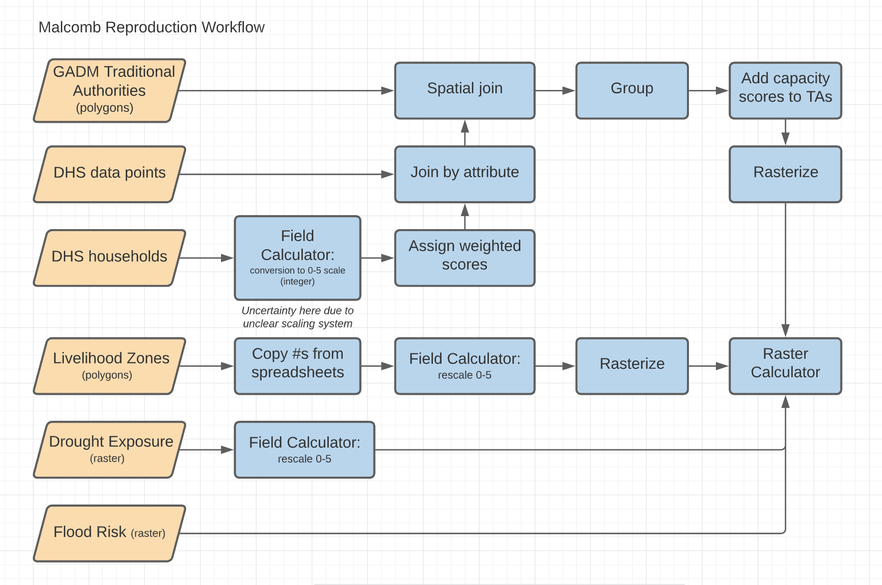
An updated workflow diagram for the reproduction of Malcomb et al. (2014). Each step of this workflow diagram represents a chunk of code in R.
Comparing outputs
In order to measure the success of our reproduction we compared our final map outputs - a map of adaptive capacity at the traditional authority level and a raster grid of overall vulnerability - to those published in figures four and five of the original study. We first georeferenced images of each of the original maps by comparing them to the traditional authorities boundaries with the georeferencing tool in QGIS 3.16. We then extracted color values from the original maps using zonal statistics. For the map of adaptive capacity by TA, we used the mean amount of red within each traditional authority to classify TAs into four resilience classes as they are presented in the original map. For the vulnerability raster, we used a vectorized raster grid with the same extent and resolution as our vulnerability output to extract the mean amount of blue in each cell, which we used as a proxy for the relative vulnerability score. To compare these maps to the outputs of our reproduction, we scaled both the digitized maps from the original study and our reproduction results from zero to one in R and calculated difference maps from them. For each pair of maps we use Spearman’s Rho value, which measures the correlation of ranked data, to assess the degree of agreement between the original maps and our reproduction results.
Reproduction Results
Our reproduction supports Malcomb et al.’s assessment of adaptive capacity at the Traditional Authority level (Figure 4 in the paper). A difference map (fig. 1) shows general agreement between our adaptive capacity map (fig. 2) and a digitized version of the adaptive capacity map presented by Malcomb et al., with most regions in our reproduction matching or being within one class break of the original value. A confusion matrix comparing the two maps (fig. 3) yielded a Spearman’s rho value of 0.77, indicating a relatively strong correlation between the original study and our reproduction. However, a high Spearman’s rho value can be achieved because the statistic is based on rank, and not value. It is possible that we would need an additional step to mask out the natural areas from this analysis, which would be an interesting step to add in a future reproduction.
We failed to reproduce the original study’s assessment of climate vulnerability (Figure 5 in the paper). There was broad disagreement between our reproduction (fig. 4) and a digitized version of the original study’s map of climate vulnerability, as shown in a map of the difference between the original study and reproduction (fig. 5). A confusion matrix comparing the two maps yielded a Spearman’s rho value of 0.15, indicating a very low degree of correlation between the original study and our reproduction. As shown in a scatterplot of vulnerability scores from the original study vs. the reproduction (fig. 6), the reproduction consistently yielded lower vulnerability scores, falling below the line of equality. Prior to comparison, the vulnerability values were scaled from 0 to 1 over the range, from minimum to maximum. As we can see in fig. 6, vulnerability scores in the original study were clustered between 0.5 and 0.9, on the high end of the range, while vulnerability scores in the reproduction were mostly distributed lower in the range, from 0.1 to 0.7. Thus, the skewness of the two distributions of vulnerability scores might explain why the reproduction was almost always lower.
Overall, the georeferencing of Malcomb et al.(2014)’s worked fairly accurately, and those that we digitized compared well with those in the original study.
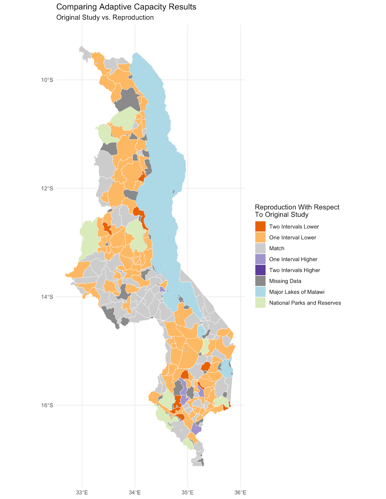
Figure 1. Map of the difference between the adaptive capacity of the reproduction vs. the original study.
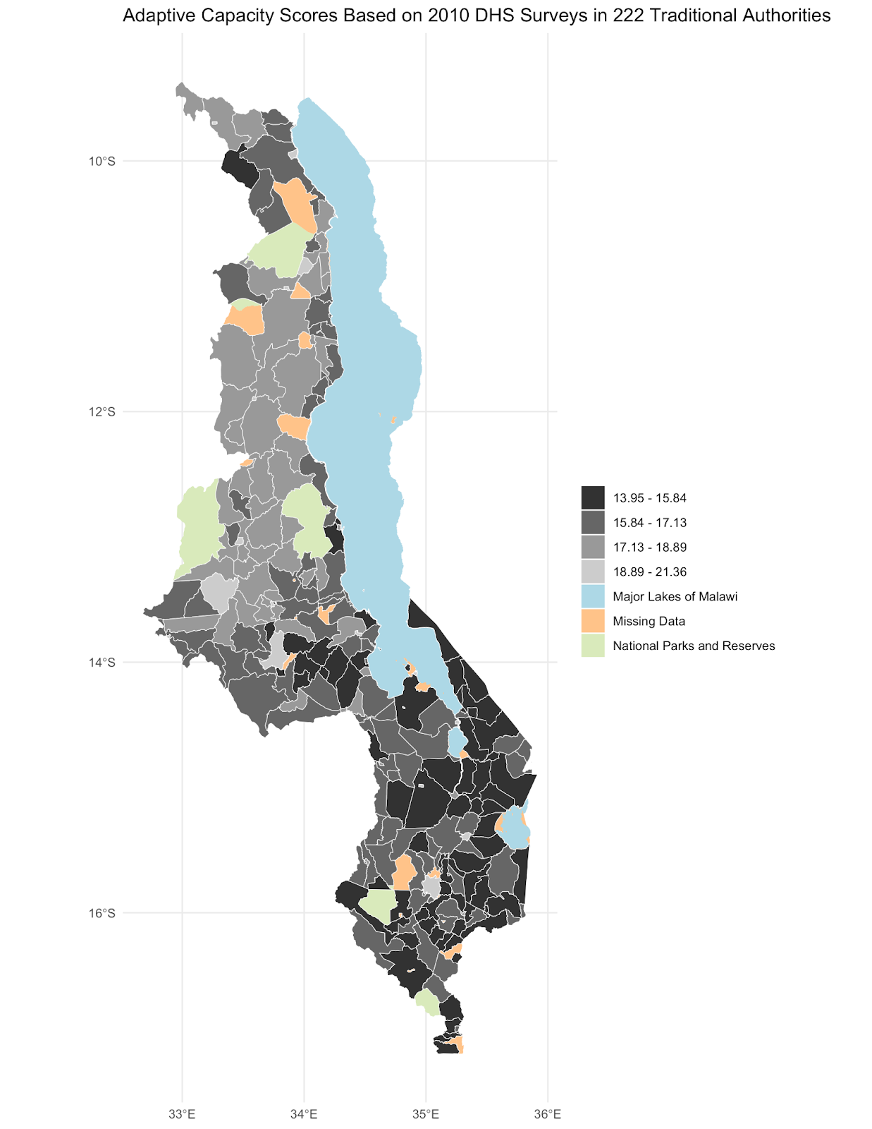
Figure 2. Reproduction results for adaptive capacity by traditional authority (TA), as calculated in R.
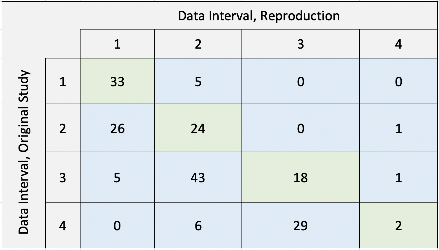
Figure 3. Confusion matrix comparing the Malcomb et al. (2014) results to the reproduction; note that the reproduction often yielded lower adaptive capacity scores than the original study, but the reproduction results for each TA were generally within one interval of the original study’s results.
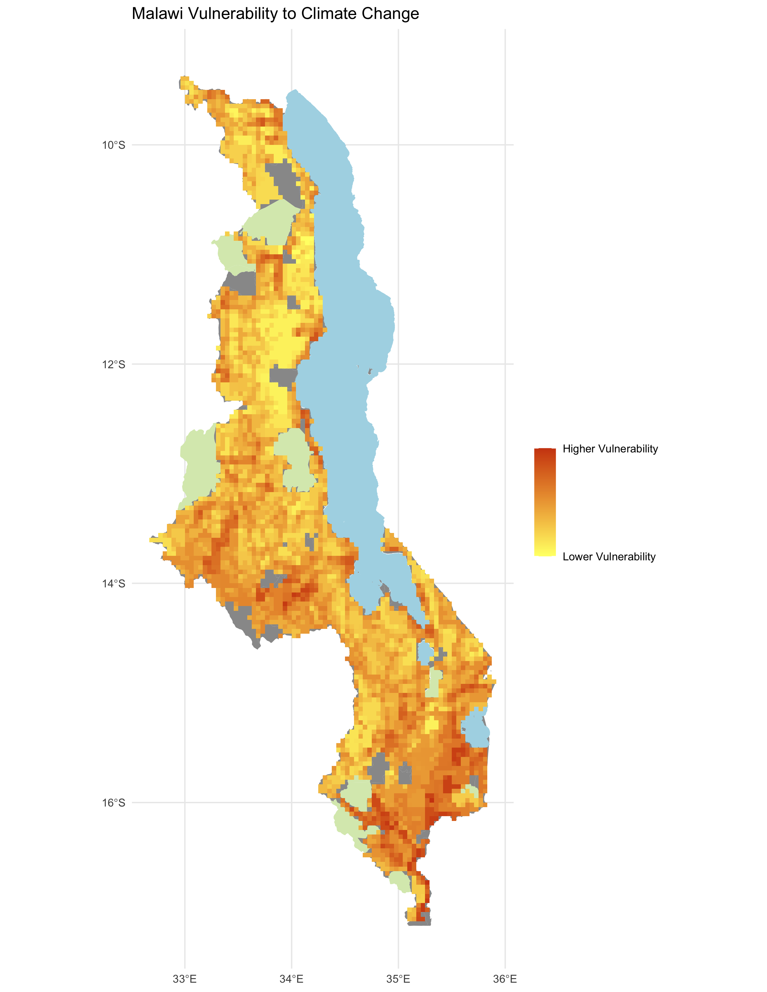
Figure 4. Reproduction results for vulnerability in Malawi, as calculated in R.
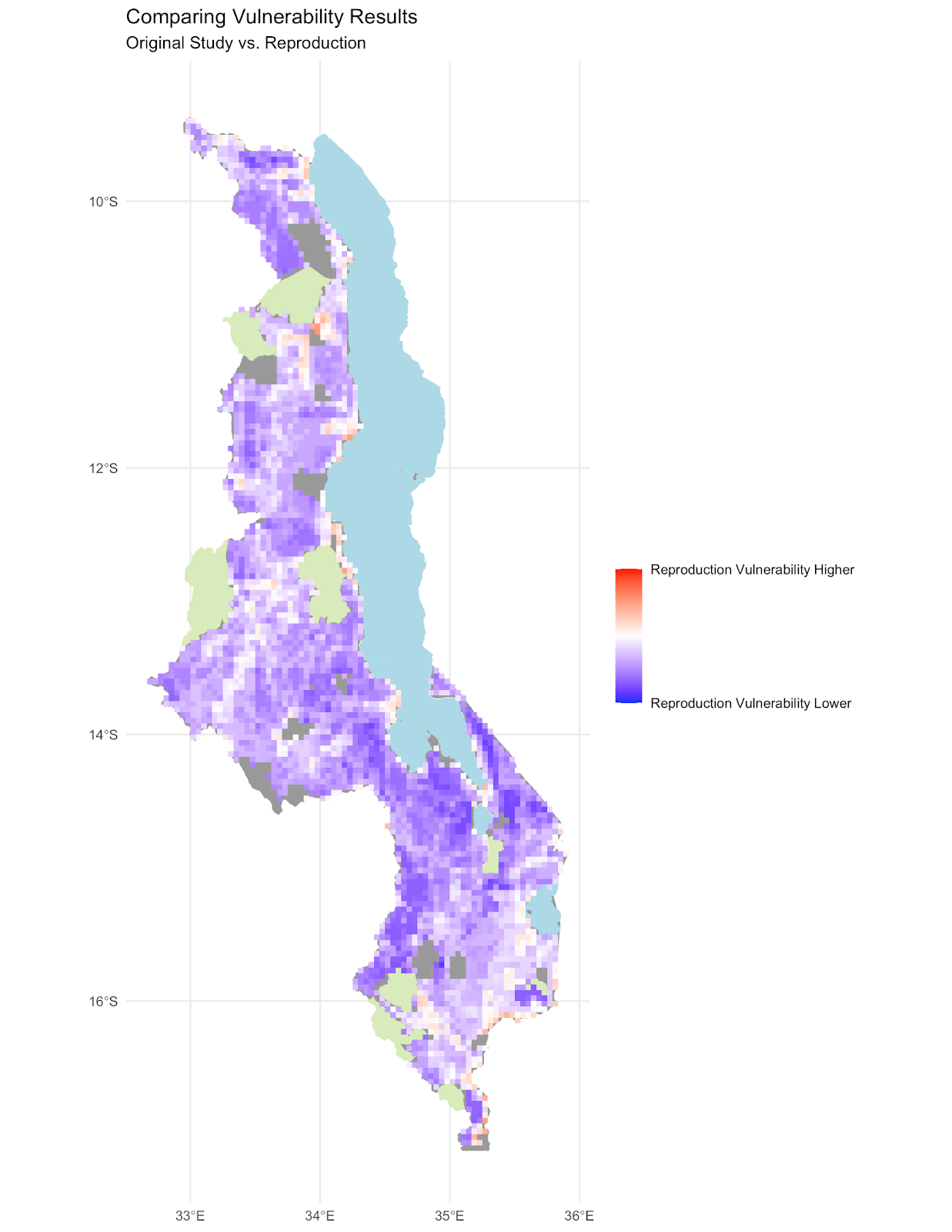
Figure 5. Map of the difference between the vulnerability calculated in the reproduction vs. the original study.
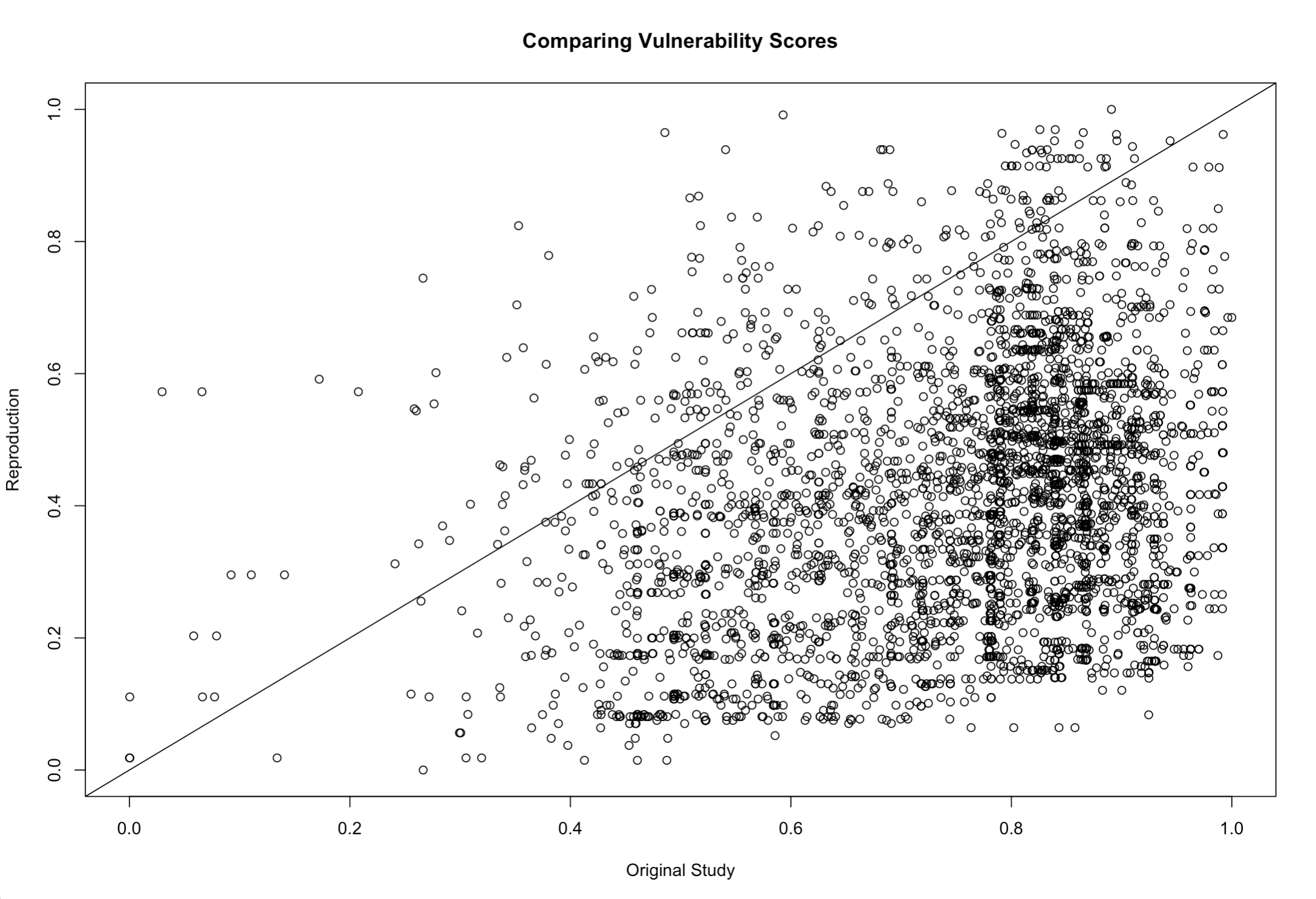
Figure 6. Scatterplot comparing vulnerability scores from the original study to the results of the reproduction.
Unplanned Deviations from the Protocol
In our initial understanding of this workflow, we planned to rasterize all of our data as our first step in order to perform the analysis. Malcomb’s methodology described the DHS indicators as “disaggregated” so we were under the impression that we needed to reduce the DHS data to the smallest scale possible. We had then planned on using zonal statistics and summarizing by region to achieve the final vectorized results. Given the ambiguous language of disaggregation, we were uncertain about the scale at which to conduct the bulk of our analysis. Malcomb’s methodology also included contradictory language about the normalization of the DHS indicators. Malcomb described the indicators as ranging from “zero representing the worst condition for a household and five being the best” but then goes on to refer to “quintiles” of households, making it unclear whether or not the DHS indicators were normalized into five or six categories (Malcomb et al. 2014).
Upon a closer inspection of the data, our main source of uncertainty centered on how to numerically quantify the “disaster coping strategy” component of the livelihood sensitivity score. The closest thing Malcomb gives to a description is the “use of natural resources for coping with disasters” (Malcomb et al. 2014). We chose to quantify this using the self-employment source of income category in the FEWSNET data and categorized anything that seemed like “use of natural resources,” such as charcoal production, firewood, grass, and the sale of wild foods. However, this is a pretty large source of uncertainty in our analysis because we have very little information as to how Malcomb quantified this factor of livelihood sensitivity.
Discussion
While we had some success reproducing Malcomb et al.’s classification of adaptive capacity, our attempt to reproduce the original authors’ assessment of climate vulnerability encountered significant challenges, largely stemming from the lack of code or a clear workflow in the original report. Inconsistencies and vagueness in the writing of the original report exacerbated the uncertainty introduced by the lack of code or workflow. Finally, in trying to reconstruct the authors’ definitions of livelihood sensitivity indicators we found significant concerns with the original study’s use and representation of that data.
As discussed above, our reliance on the authors’ ambiguous narrative description of their methods rather than code or a workflow diagram was a significant source of uncertainty on our reproduction methods. Even with access to complete data and a description of each indicator used to calculate adaptive capacity, we were unable to match the original results exactly. Although Table 1 in the original report provides a description of each indicator, it provides neither the exact variables used to construct each indicator nor the manner in which these variables were combined to form the indicators (Malcomb et al. 2014). The methods used to scale these variables were also unclear and at times contradictory, leaving us to guess which variables to include and how to aggregate and scale them. In a case like defining variables for the ‘livestock’ indicator this was not a significant challenge, but the discrepancy in how the authors describe their scaling method was a source of confusion when we were constructing our workflow and could have had a significant impact on the results, as did the lack of a clear definition of “disaster coping strategy.” This caused subjective differences in our workflows. As stated by Tate, subjectivity is not inherently a bad thing, and is necessary to some degree in modelling efforts (Tate 2013). However, it is important to address these differences that stem from the lack of a clear methodology. It was also unclear exactly how the authors converted the household resilience score, in which higher values represent lower vulnerability, into the vulnerability score shown in Figure 5 of the original report, and we again had to infer this methodology from our own understanding of the data and the parts of the workflow that we understood better. Including the analysis code or workflow models in the original report would have eliminated all of these sources of uncertainty and could have led to a much more robust reproduction.
Additionally, the original authors’ presentation of the FEWSNET livelihood zones at best overestimates and at worst misrepresents the actual content and reliability of that data. They refer to the livelihoods zones data as a “countrywide survey” (pg. 21) and weight the indicators derived from it similarly to those derived from DHS data, but the livelihood zones data are not derived from surveys in the same way that the DHS data are (Malcomb et al. 2014). The FEWSNET data were created from focus group consultations in four villages and two districts in each zone, which were selected based on interviews with district-level government officials and NGOs (“Guidance Notes for Livelihood Zones” 2005). Put simply, these data were constructed from a small, normative sample of the population of a small, normative sample of the villages within each livelihood zone. While the organization into non-administrative livelihoods zones may be accurate and this data may have important applications, using it as a vital input to a fine-resolution assessment of climate vulnerability seems to grant it more credibility and geographic specificity than it deserves.
Furthermore, it was sometimes unclear how the authors used the FEWSNET data on livelihood zones, because they included relatively little discussion of the variables in question – percent of food from one’s own farm, percent of income from wage labor, and percent of income from cash crops. A careful reading of the paper suggests that Malcomb et al. frame the first two as positive and the third as negative, but there is some uncertainty here, and our reproduction may have reversed the direction of one of these variables, explaining some of the divergence between the reproduction results and the original study.
It is also important to reiterate the levels of uncertainty apparent in all geographic representations (Longley et al. 2005). The data used for the replication is based on a specific conception of the real world, and each of the various data sources have a specific level of error within them. Furthermore, the aggregation of data from the household level into the village level, and later into traditional authorities can lead to uncertainty in representation.
Conclusion
The levels of difference between the Malcomb et al. study and our reproduction (illustrated by the difference maps and our reproduction figures) emphasize an important key finding, that studies must provide clear workflows, methodologies, and data transparency in order for reproductions to occur. While our final visuals do serve as a representation of greater areas of adaptive capacity, the levels of uncertainty stemming from issues in the data and methods make it so that our work was unable to fully match that of Malcomb et al. With increased transparency and details in the field of climate change modeling, this will lead to improvement for all future models.
The research findings suggest a need for further exploration of climate change vulnerability, and the ways that vulnerability and climate change risk are measured and quantified. Future research should continue to consider new available datasets that may contribute to a greater understanding of risk, at a variety of scales. Additionally, it is important to consider the broader societal implications that can occur from the labeling of certain regions as the most vulnerable to climate change. We can also consider the ways that Malcomb et al. and our reproduction connect to a greater pool of climate change adaptation and development theory. In Mark Pelling’s theory of climate change adaptation and development, he emphasizes the importance of empowering the most vulnerable populations, which includes processes such as taking local voices into consideration in the policy making process, and considering the potential socio-political factors that make these populations vulnerable without placing the blame on these groups (Pelling 2011). However, oftentimes labeling a specific community or spatial region as highly vulnerable can be disempowering, potentially creating a narrative that this area is already too prone to risk to be saved by new climate policy.
The mapping of vulnerability, or any data that reflects the unequal distribution of risk across space, is crucial for considering where support should be directed. Future research, however, should also work to account for vulnerability at different scales, and new time periods. The results and implications of the current vulnerability maps produced by Malcomb et al. are important starting points for considering spatial variation in vulnerabilities, however they reflect data from a poorly defined time period, and new temporal data will continue to strengthen the models. And while quantitative models such as this one are crucial for identifying areas of risk, the aggregation of data into villages, traditional authorities, or livelihood zones must be viewed as an average result, as it does not account for the various unique vulnerabilities that individual households may face.
References
Longley, Paul, ed. 2005. Geographical Information Systems and Science. 2nd ed. Chichester ; Hoboken, NJ: Wiley.
Malcomb, D. W., E. A. Weaver, and A. R. Krakowka. 2014. Vulnerability modeling for sub-Saharan Africa: An operationalized approach in Malawi. Applied Geography 48:17–30. DOI:10.1016/j.apgeog.2014.01.004
Pelling, Mark. 2011. Adaptation to Climate Change: From Resilience to Transformation. London ; New York: Routledge.
Tate, E. 2013. Uncertainty Analysis for a Social Vulnerability Index. Annals of the Association of American Geographers 103 (3):526–543. doi:10.1080/00045608.2012.700616.
Report Template References & License
This template was developed by Peter Kedron and Joseph Holler with funding support from HEGS-2049837. This template is an adaptation of the ReScience Article Template Developed by N.P Rougier, released under a GPL version 3 license and available here: https://github.com/ReScience/template. Copyright © Nicolas Rougier and coauthors. It also draws inspiration from the pre-registration protocol of the Open Science Framework and the replication studies of Camerer et al. (2016, 2018). See https://osf.io/pfdyw/ and https://osf.io/bzm54/
Camerer, C. F., A. Dreber, E. Forsell, T.-H. Ho, J. Huber, M. Johannesson, M. Kirchler, J. Almenberg, A. Altmejd, T. Chan, E. Heikensten, F. Holzmeister, T. Imai, S. Isaksson, G. Nave, T. Pfeiffer, M. Razen, and H. Wu. 2016. Evaluating replicability of laboratory experiments in economics. Science 351 (6280):1433–1436. https://www.sciencemag.org/lookup/doi/10.1126/science.aaf0918.
Camerer, C. F., A. Dreber, F. Holzmeister, T.-H. Ho, J. Huber, M. Johannesson, M. Kirchler, G. Nave, B. A. Nosek, T. Pfeiffer, A. Altmejd, N. Buttrick, T. Chan, Y. Chen, E. Forsell, A. Gampa, E. Heikensten, L. Hummer, T. Imai, S. Isaksson, D. Manfredi, J. Rose, E.-J. Wagenmakers, and H. Wu. 2018. Evaluating the replicability of social science experiments in Nature and Science between 2010 and 2015. Nature Human Behaviour 2 (9):637–644. http://www.nature.com/articles/s41562-018-0399-z.
Acknowledgments
Thanks to Emma Brown for substantial revisions to this report.
 This work is licensed under a Creative Commons Attribution-NonCommercial-ShareAlike 4.0 International License.